P-hacking

The picture above says it all !! Since ages right from the era of the great Mr. Sherlock Holmes we know the importance of data. Not only a dump of data but the data collected should be of superior quality to reduce the pure error.
But do you really think that the data with P-Value within the limits of significance is good enough ? Well the concept of p- Hacking will definitely make you think twice about this.
Now let’s take a quick snapshot of what P-value is before jumping onto P hacking !!
A p value is used in hypothesis testing to help you support or reject the null hypothesis. The p value is the evidence against a null hypothesis. The smaller the p-value, the stronger the evidence that you should reject the null hypothesis.
A small p (≤ 0.05), reject the null hypothesis. This is strong evidence that the null hypothesis is invalid.
A large p (> 0.05) means the alternate hypothesis is weak, so you do not reject the null.

Having P value within the limits of significance doesn’t guarantee the correctness.
It is usual and always the case where an increment in sampling size might reduce the risks, but it is not always true.
With an increase in sampling size, risks might also increase. A better model which would be more complex and accounts for co-variation should be used for data analysis.
No steps can guarantee an absolute elimination of data dredging but it can be certainly reduced to the level where it becomes insignificant.
Let’s take an example of covid 19 data. When we did not have any specific drug on disease and scientists were experimenting and we were looking for results…. Which vaccine performed well… what is accuracy… n ol….
Taking in consideration the performances of the vaccine, we decided which one we will take. Now the next question arises… how do we calculate this accuracy? What if it does not go well…… ?
Should we believe in these results ?
To confirm our beliefs technically and statistically the best rescuer is P-hacking and methods to avoid it.
We have Pfizer, Moderna, Oxford/AstraZeneca, COVEXIN… n so on and let’s test them for accuracy. { For this blog,instead of taking actual names,we have taken the names line vaccine A , vaccine B ……., vaccine Z}
Let’s have 3 people without being vaccinated and have a set 3 people to be vaccinated with vaccine A to Z respectively.
Comparing them doesn’t seem like vaccine A is that effective. So we will continue the vaccine B, Vaccine C, vaccine D…. until we get satisfying results. And at last we got great results for vaccine Z. { Ref the Fig A below }

So we calculate the mean of two groups ( one not vaccinated and other vaccinated ) and perform a statistical test to compare the mean…resulting P-value = 0.02.
As 0.02<0.05 we reject the null hypothesis which means there is a difference between not taking vaccine and taking vaccine Z
Are we getting the correct result or are we getting fooled / misled ? Or precisely are we just P-hacked?
P-hacking refers to the misuse and abuse of analysis techniques and results in being fooled by false positives. You must be wondering how this happend? Don’t worry…. We will learn what P-hacking is. So that we can avoid getting P-hacked.
Let’s take both samples from the same distribution. If we take two sets of three people and ask them about getting an infection and plot them on a graph with respective mean. We do a test to compare the two mean and get P-value= 0.65. As 0.65>0.05, we would fail to see a significant difference between two sets of people. And this is right because both samples are from the same distribution.
If we continue taking two sets of three people from the same distribution and calculate p-value to see if they are different until we get p-value<=0.05. After so many sets, finally these two sets look different but P-value = 0.02. Which is less than 0.05. And that tells us that there is a statistically significant difference between two sets of people. So these two sets are from two different distributions. But actually this is incorrect because we took sets from the same distribution. This P-value is false positive.
Now let’s learn a few things about false positives. Whenever we talk about normal distribution, we set a threshold of significance which is our P-value= 0.05. Meaning that approximatally 5% of the total data will result in false positives. Suppose we did 100 tests that resulted in 5 false positives… 50 in 1000 … 500 in 10000 … large tests will result in large false positives.
This is known as the Multiple Testing problem. To deal with this problem we will use one of the popular methods named FDR (False Discovery Rate). Another method is The family-wise error rate (FWER). This blog is focused on FDR only.
FDR
Whenever we get hacked or fooled… FDR is savier.. This helps us to identify false data which looks good.
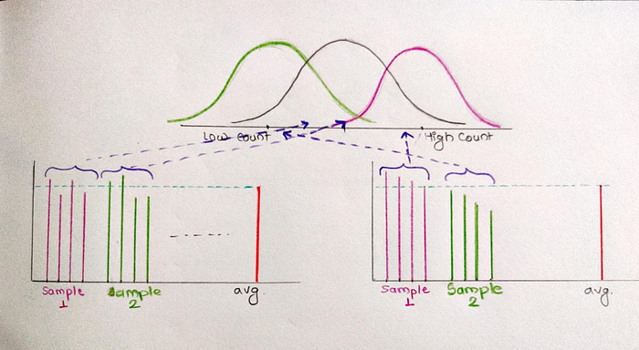
Let’s take an example, Measuring human gene expression with RNA-seq. We will count a particular type of gene i.e gene A from a sample of normal people and people who took the vaccine. If we take the average of gene A count for all, we will observe that most of the values are close to mean. In rare conditions we will get values which are much larger and smaller than mean.

Now we will try to fit all values in the normal distribution/ bell shaped curve. For that make sample_1 (group of 4 people) and do RNA-seq.
As these values are close to the mean, they are from the middle of the distribution. Now if we compre sample_2 (group of 4 people), they are also from the middle of the distribution.
If we do statistical tests to compare both the samples, the P-value will be larger as they are from the same distribution and closer to the mean. Very rarely we will get a P-value less than 0.05 may be because samples are not overlaped. This is called false postive.
FDR can control the number of false positives. Particularly it is used for the ‘Benjamini-Hochberg method’.
Additional information : There are other method of FDR like Benjamini-yekutieli, Stotrey’s pFDR and Combined prob Fisher
What is this Benjamini-Hochberg method?
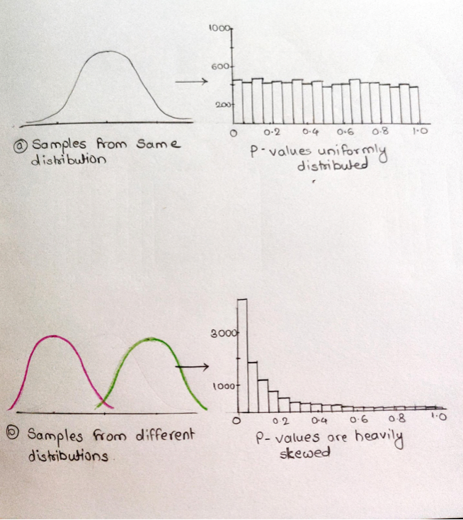
For that we will start with an example, we will do a statistical test to get 10000 p-values from the same distribution(normal people). In this case all P-values will be greater than 0.05. And draw a histogram of all P-values with around 500 bin sizes. P-values are uniformly distributed. Similarly, we will do a statistical test to get 10000 p-values from the different distributions(vaccinated people). For diffrent distributions all P-values will be less than 0.05 as expected. When we draw a histogram for these P-values, we get a different distribution of P-values (Heavily left screwed). Most of the P-values are less than 0.05. On the other side P-values> 0.05 are false negatives.
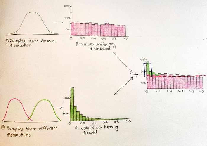
We can reduce false negative values by increasing sample size. From 10000 people, 1000 are vaccinated and 9000 are normal people. Histogram of P-values obtained from all 10000 is sum of two separate histograms. By eye we can see where the P-values are uniformly distributed and determine how many tests are in each bin. When we extend this line and use it as a cut off to determine the ‘True positives’. Since we usually use cut off 0.05, we are going to focus on these values. Roughly 450 P-values<0.05 are above the dotted line and 450 P-values<0.05 are below. To stay away from false positives, it would be great if we use only the smallest P-values. This is what we do in the Benjamini-Hochberg method but in a mathematical way. It adjusts P-values in a way that limits the false positives that are reported as significant.
What are adjusted P-values?
Suppose, before doing FDR correction, our P-value might be 0.04 which is significant. And after the FDR correction, our P-value might be 0.06 which is not significant.
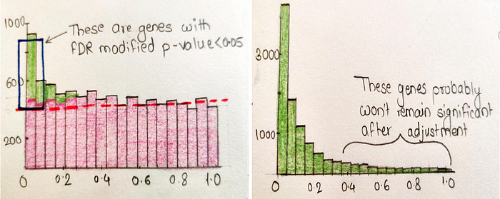
In above fig notice that not all of the ‘true positive’ genes are inside the box. Only 5% of them are false positives, the other 95% are true positives. Because not all true positives will have super small P-values. This is all about the Benjamini-Hochberg method therotically, now let’s have a look at the mathematical side.
Let’s take a sample of 5 normal people from the same distribution. These are the p-values for the same [0.03, 0.21, 0.46, 0.72, 0.87].
Steps -
- Arrange the P-value in ascending order
- Rank them in ascending order
- Calculate adjusted P-value
- For last one P-value and adjusted P-value are same
- For second last adjusted P-value… is smaller of two option: either the previous adjusted P-value OR
Current P-value *(total no. of P-value/ P-value rank)
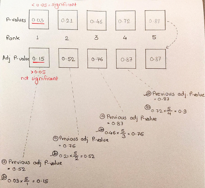
First P-value is false positive which is no longer significant in adj P-value. To get Adj P-value properly we have to take in consideration all P-values instead the one which looks like it will give us a small P-value.
This is one way of getting hacked, we will discuss another way of P-hacking. For a particular set where we were getting P-value = 0.06. In reality these groups are coming from the same distribution but while testing we don’t know if it is from the same or different distribution.
And Obviously we hope that they are from different distributions. So when we get P-value = 0.06, which is slightly greater than 0.05. Now it is very obvious to think that if we add more data, the P-value will get smaller. So let’s try this, When we add one sample(a set of four people instead of three) in both sets. And calculate P-value, we get 0.03 which is less than 0.05.
Great… Now we can say these sets are from different distributions. But Is it really correct? NO… We are P-hacked again. When adding data this results in false positives. How can we avoid making this mistake ?
We need to determine the appropriate sample size which is known as Power Analysis. Power analysis can be used to calculate the minimum sample size required so that one can be reasonably likely to detect an effect of a given size and correctly reject the null hypothesis.
Keep watching this space for the next series of blogs on Power Analysis !!
